Image Super-Resolution
deep learningزيادة أبعاد الصورة عن طريق الـ
Image Super-resolution (SR) هو الإسم المتداول لعملية تحويل الصورة من Low resolution إلى high resolution عن طريق زيادة عدد الـpixels في الصورة بحيث تحافظ على التفاصيل الموجودة فيها، وهي من أكثر التقنيات أهمية في مجال الـImage processing والـcomputer vision وتدخل في العديد من التطبيقات في الواقع زي تحسين الصور الطبية (Medical Imaging) وصور الأقمار الصناعية وكاميرات المراقبة الـlive-streaming وغيرها الكثير.
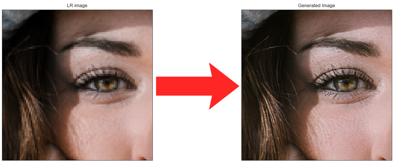
Fig 1: Original low-resolution image (right) and its generated high-resolution (Super resolved) counterpart (left)
ممكن نمثل عملية الـsuper resolution عن طريق الـdiagram الموجود في Figure 2، الـdiagram بيوضح إن الصورة الـlow resolution جاية عن طريق تطبيق عملية downsampling على صورة high resolution بالإضافة لبعض الـnoise، فبالتالي أي موديل هنعمله بيحاول يتعلم يعكس العملية دى عشان يوصل من الـlow resolution للـhigh resolution.
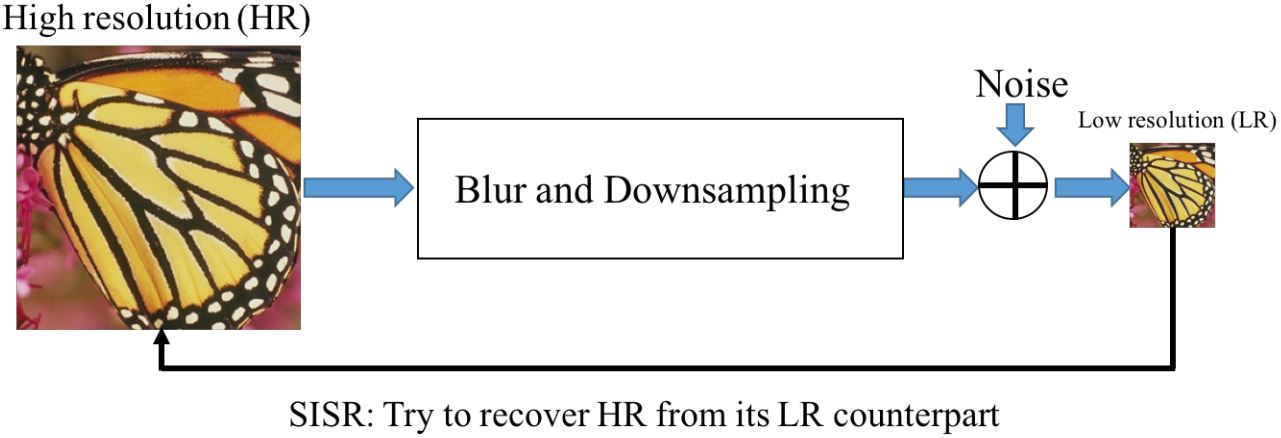
Fig 2: Sketch of the overall framework of SISR
Source: Click here
التحدي في مشكلة الـsuper resolution هو أنها تعتبر ill-posed problem، بمعنى إن فيه عدد كبير من الصور الـhigh resolution ممكن تطلعه من أي صورة low resolution، ومفيش أي طريقة متاحة تقدر تحكم بيها وتقول مين أفضل واحدة إلا لو معاك الصورة الـhigh resolution الأصلية، لذلك في الـproduction مفيش metric ممكن تتابعه وتحكم على آداء الموديل من خلاله.
الطرق التقليدية في الـsuper Resolution
الـsuper resolution كان موجود من فترة كبيرة في الـimage processing قبل حتى قدوم الـdeep learning للساحة تحت مسمى image interpolation، فيه أكثر من طريقة ممكن نعمل بيها interpolation زى الـnearest neighbour، bilinear، bicubic interpolations، الطرق دى بتتنفذ بمعادلات رياضية مباشرة ومش بتحتاج تتعلم أي parameters قبل ما تشتغل، وبالرغم من إنها سريعة ومباشرة إلا إن نتايجها كان غير مرضية وقد تكون غير مقبولة.
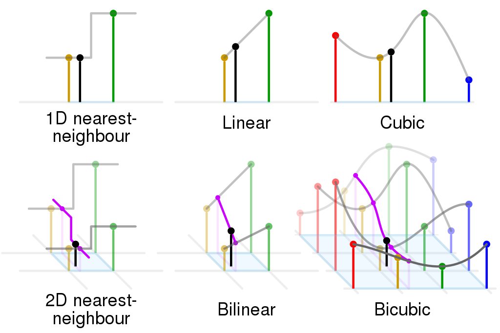
Fig 3: Comparison between NN, Bilinear, and Bicubic Interpolation
Source: Click here
استخدام الـdeep learning في الـsuper resolution
أول محاولات تطبيق الـdeep learning في الـsuper resolution كانت في 2014 عن طريق SRCNN Model، الموديل البسيط الموضّح في figure 4 بياخد ناتج أحد الطرق التقليدية زى الـbicubic interpolation ويمرره على 3 conv layers عشان يحسن نتيجته.
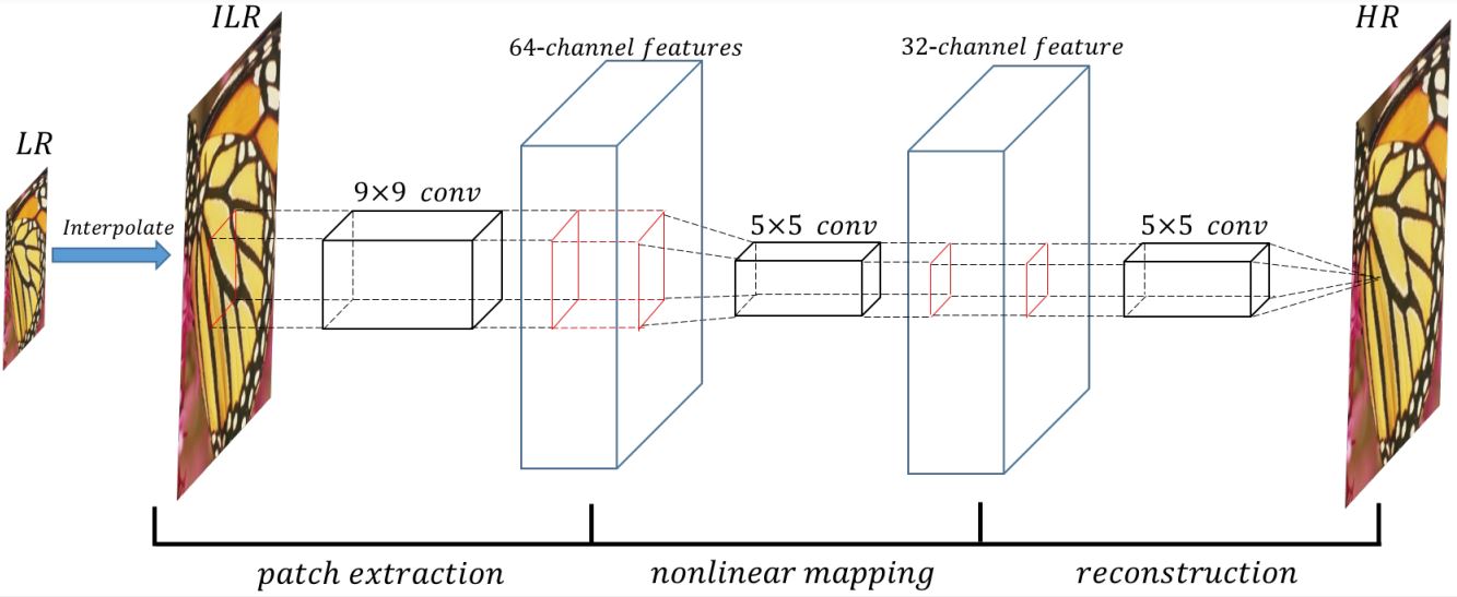
Fig 4: Sketch of the SRCNN architecture
Source: Click here
الموديل بيستخدم mean square error كـloss function وقدر يحقق state of the art results في وقت ظهوره في 2015 لكنه يحتوي بعض العيوب:
- استخدام bicubic interpolation بينتج smooth images وبالتالي الموديل مش بيقدر يتعلم الـdetails الموجودة في الصورة وممكن يؤدي إلى نتايج غير مرضية.
- استخدام اي نوع من الـinterpolation بيقيد آداء الموديل بشكل كبير، لإنها بتفترض إن كل الصورة low resolution بتكون ناتجة من نفس الـdownsampling operation لكن في الواقع ده غير صحيح.
- الموديل بيشتغل على صورة بحجم الـhigh resolution وهي 4 أضعاف حجم الـlow resolution (لو إفترضنا إن الـscaling factor=4) وبالتالي عدد الـoperations الى الموديل بينفذها بيزيد بشكل كبير جداّ مع زيادة حجم الـlow resolution image.
أحد حلول المشاكل دى هو إننا نعمل upsampling في آخر الموديل، ويكون عن طريق trained weights بدل الطرق التقليدية، كده الموديل يقدر يتعلم الـupsampling الى هو محتاجه وبالتالي تفاديت قيود الـinterpolation، وكمان الموديل دلوقتي بيتعامل مع الصورة الـlow resolution بس وبالتالي عدد الـoperations الى بيعملها أصبح أقل.
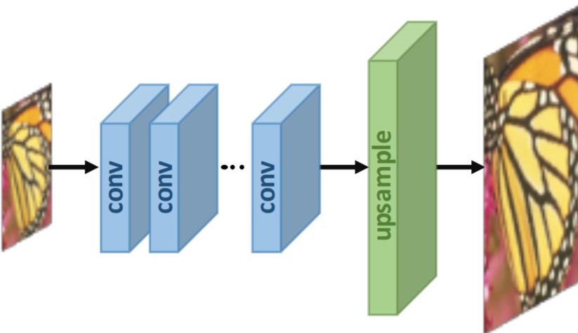
Fig 5: Post-upsampling Technique
Source: Click here
طرق الـupsampling المستخدمة في الـdeep learning
الطريقة الأولى تتم باستخدام deconvolution layer أو transposed convolution layer، وفيها بنعمل upsampling للـinput feature map عن طريق nearest neighbour وبعدها نمررها على convolution layer (لاحظ Figure 6)، كده نقدر نسخدم learnable weights في الـupsampling وكمان أصبحت العملية أسرع لإن الـnearest neighbour upsampling بسيط ومفيش فيه أي حسابات.
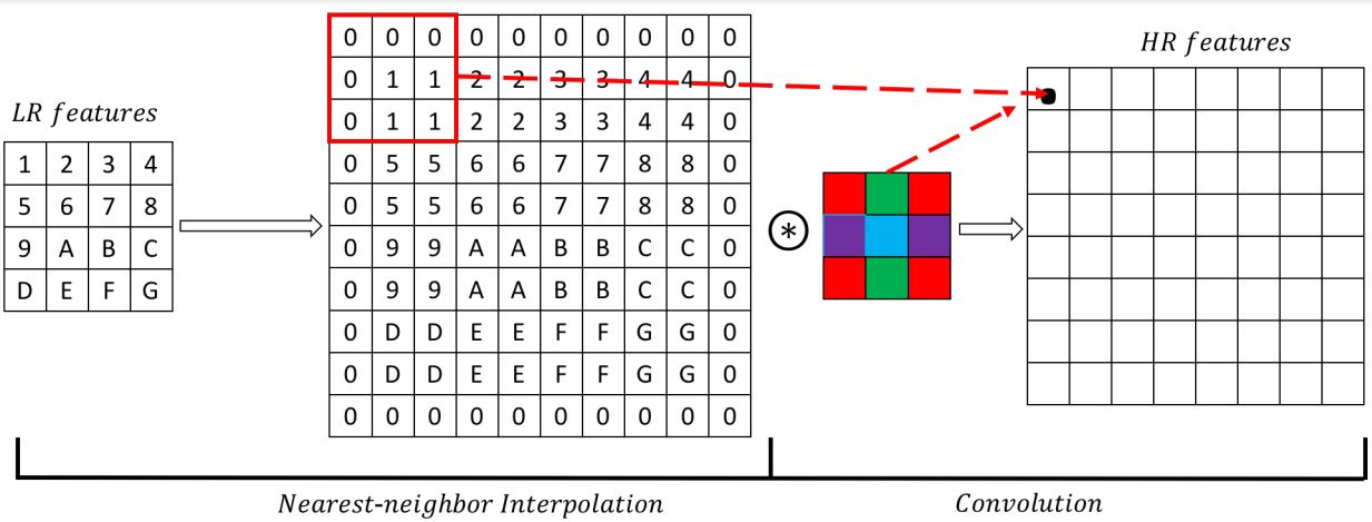
Fig 6: Sketch of the deconvolution layer
Source: Click here
المشكلة في الـdeconvolution layer هى إن الـnearest neighbour بيكرر الـpixels الموجودة في الـfeature map وبالتالي بيضيف نوع من الـredundancy وده بيأثر على جودة الـoutput الناتج من الموديل، لذلك ظهرت طريقة آخرى للـupsampling تعتمد بشكل كامل على learnable weights وفي الـefficient sub-pixel convolutions (ESPC)، الفكرة منها هو إن لو عايز أكبّر الصورة ب$factor=r$، هستخرج feature maps عددها $r^{2}$، وأرتّب الـpixels المناظرة من كل feature map جنب بعض كما هو موضّح في Figure 7.
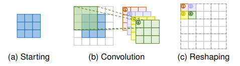
Fig 7: Sub-pixel convolution layer with a scaling factor=2
Source: Click here
الـmodels المستخدمة في الـsuper resolution
مع استخدام الـdeep learning في الـsuper resolution ظهرت models وarchitectures كثيرة جداً، بعض الأمثلة موضّحة في Figure 8. كل واحد منهم محتاج مساحة غير صغيرة من المقال لتغطية تفاصيله لذلك هكتفي بالاتنين الى طبقتهم وهم SRResNet و الـEDSR.
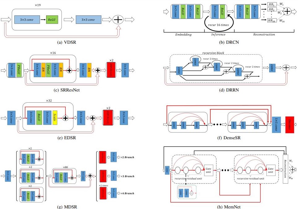
Fig 8: Sketch of several deep architectures for SISR
Source: Click here
SRResNet Model
الـResNet architecture قدمت حل سحري لمشكلة الـvanishing gradients وأتاحت لنا القدرة على تدريب deep models بدون مشاكل، الـSRResNet بتتبنى نفس الفكرة مع بعض الإضافات لتلائم الـsuper resolution، كما هو موضح في figure 8 (c)، الموديل مكوّن من 16 residual block، كل block يحتوى على اتنين conv layer واتنين batch normalization layer بينهم Parametric ReLU، وفي الـoutput بيستخدم اتنين ESPCN بـscaling factor 2 عشان يضاعف حجم الصورة 4 مرّات، وبيستخدم mean square error loss function موضّحة كالآتي:
$$
l_{MSE} = \frac{1}{r^{2}WH}\sum^{rW}_{x=1}\sum^{rH}_{y=1}(I^{HR}_{x,y} - I^{SR}_{x,y})^2
$$
حيث H,W هما طول وعرض الصورة الـlow resolution، وr هو الـscaling factor، و $I^{HR}$ هي الصورة الـhigh resolution الأصلية، و $I^{SR}$ هي الصورة الناتجة من الموديل.
لو عايزين نبني الموديل بالكود، في البداية هعمل function بتبني الـresidual block:
|
|
بعد كده هنعمل الـupsampling operation، لكن keras مفيش فيه ESPCN layer لذلك هنسخدم conv layer عادية ونعمل بعدها pixel shuffle عن طريق depth to space layer الموجودة في tensorflow:
|
|
الآن هنبني الموديل بالكامل، ممكن تراجع الـdiagram الخاص بالموديل من الـpaper بتاعته، والموضّح في Figure 9:
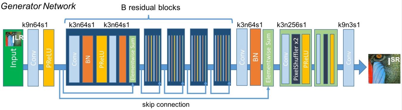
Fig 9: SRResNet Model Architecture as described in paper
Source: Click here
|
|
ممكن تشوف كود الموديل بالكامل هنا.
الـSRResNet قدر يحقق نتائج ممتازة بفارق كبير عن الطرق السابقة، لكن تظل مشكلة واضحة في الـoutput الخاص بالموديل وهو إنه رغم تحقيقه لنتائج ممتازة جداً في الـPSNR والـSSIM إلا إن الصورة بيظهر فيها نوع من الـblurring effect.
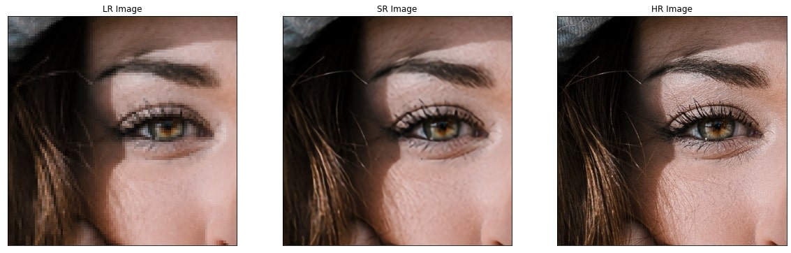
Fig 10: SRResNet Output (middle) compared to input (left) and original (right)
EDSR
في 2017 ظهر موديل جديد اسمه Enhanced Deep Super-Resolution Network (EDSR)، في الـPaper دى بيقترحوا تعديل في تصميم الـSRResNet وذلك عن طريق استبدال الـPReLU بـReLU والاستغناء عن أي activations خارج الـres block والاستغناء عن الـBatch norm layers تماماً من الموديل. الـPaper بتبرر التعديل ده بإن الـResNet مصممة لحل high level problem وهي الـClassification، في هذا النوع من المشاكل الـshift الناتج من استخدام الـBatch norm ليس له تأثير واضح على دقة الـoutput، أما في حالة low level problems زى الـsuper resolution، فالـinput والـoutput مرتبطين ببعض بشكل كبير وبالتالي الـbatch norm بيأثر على جودة الـoutput.
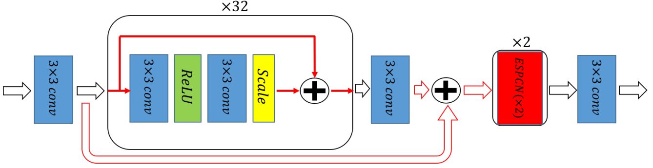
Fig 11: Sketch of EDSR Model
Source: Click here
لكن الـbatch normalization بيديني ميزة مهمة جداً وهي الـtraining statibility، هل أقدر أدرّب الموديل بدونه؟
الـPaper بتقول إن تصميم الموديل بـ16 res block هيقدر يخلينا ندرّبه بدون مشاكل، لكن لو حبينا نعمل موديل أكبر (زى الموضّح في Figure 11) فممكن نعمل scaling للـfeature maps داخل الـres block، ده هيعوّض بعض التأثير الى فقدته لما استغنيت عن الـbatch norm
التعديل ده رغم إنه بسيط لكن الإستغناء عن الـbatch norm layers أدى إلى إن الموديل أصبح يستهك 40% memore أقل من الـSRResNet، وبالتالي أصبح الـEDSR بياخد تقريباً نص الوقت الى كان بياخده الـSRResNet في كل Epoch بنفس الـbatch size، بالإضافة إلى إن لو معايا GPU بـmemory كبيرة فممكن استخدم batch size أكبر وأحصل على training time أقل كمان.
التعديل الثاني هو استبدال الـmean square error بـmean absolute error كـloss function، الـPaper بتبرر التعديل ده بإن الـMAE يؤدي لـbetter convergence near the minimum ولذلك يصل لنتائج أفضل.
$$ l_{MAE} = \frac{1}{r^{2}WH}\sum^{rW}_{x=1}\sum^{rH}_{y=1}|I^{HR}_{x,y} - I^{SR}_{x,y}| $$كود الـEDSR بسيط ومشابه إلى حد كبير للـSRResNet، الى احنا هنطبقه هنا هو الـbase model الموجود في الـpaper وهو عبارة عن 16 res block فقط وبدون scaling. الكود الخاص بالـres block والـupsample block هيكون كالآتي:
|
|
دلوقتي نقدر نبني الموديل:
|
|
تقدر تشوف كود الموديل بالكامل هنا.
الـEDSR قدر يحقق نتائج أفضل من الـSRResNet وفي وقت أقل لكن ماتزال مشكلة الـsmoothing واضحة في الـoutput. عشان نحل المشكلة دى، الـPaper الخاصة بـSRResNet أقترحت عمل fine-tuning للـweights الخاصة به عن طريق تدريبه في Generative Adversarial Network (GAN) عشان يقدر ينتج صور بتفاصيل أفضل وأكثر واقعية
SRGAN
الـPaper بتقول إن سبب الـblurring هو إن تدريب الموديل على mean square error، بينتج output عبارة عن average لأكتر من output محتمل عشان بتوصل لأقل mean square error ممكن ولكن بتسبب الـblurring الظاهر في الصورة. وبناء على كده اقترحوا طريقة جديدة لتدريب الـsuper resolution models معتمدة على GAN، وده بسبب قدرة الـGAN على توليد صور Realistic وأقرب ما تكون للصور الواقعية
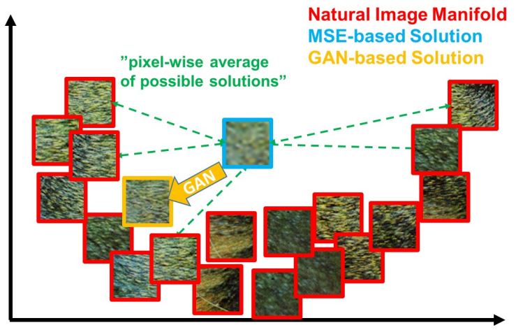
Fig 12: Illustration of patches from the natural image manifold (red) and super-resolved patches obtained with MSE (blue) and GAN (orange)
Source: Click here
تدريب الموديل في GAN هيساعده في توليد تفاصيل أكثر في الصورة بفضل الـfeedback الى هياخده من الـdiscriminator، لكن بعكس تصميم الـGANs المعتاد وهو إن الـgenerator loss معتمدة على الـdiscriminator فقط، هنا لازم الـgenerator ياخد feedback مباشر عن الـoutput بتاعه، لإن انا مش مهتم فقط بإنه يطلع realistic images، ده لازم تكون الصور الناتجة محافظة عن نفس الـcontent الموجود في الصورة الأصلية، لذلك فالـgenerator loss هنا مكوّنة من جزئين:
- Adversarial loss: ده الجزء الخاص بالـfeedback الجاي من الـdiscrimator; وده بيحكم على قدرة الـgenerator على خداع الـdiscriminator ومعادلته كالآتي:
$$
l_{Gen} = \sum^{N}_{n=1}-log(D(I^{SR}))
$$
حيث أن $D(I^{SR})$ هو output الـdiscriminator بالنسبة للـgenerated image
- Content loss: وده الجزء الخاص بالـcontent الموجود في الصورة الأصلية، الpaper هنا بتقول إن استخدام mean square error كـcontent loss مش بيقدم نتيجة كويسة ولذلك أستخدموا VGG loss: بدل ما نعمل mean square error على الصور بشكل مباشر، هندخل الصور على pretrained VGG19 network عشان تستخرج high level features ونحسب عليهم الـmean square error. معادلة الـVGG loss موضّحة كالآتي:
$$
l_{VGG/i,j} = \frac{1}{r^{2}W_{i,j}H_{i,j}}\sum^{rW_{i,j}}_{x=1}\sum^{rH_{i,j}}_{y=1}(\phi_{i,j}(I^{HR})_{x,y} - \phi_{i,j}(I^{SR})_{x,y})^2
$$
حيث أن $\phi_{i,j}$ تدل على الـfeature map الناتجة من الـconvolution رقم j وقبل الـmaxpooling رقم i في VGG19 network
الـgenerator loss (وتسمى هنا perceptual loss) هتكون عبارة عن weighted sum بين الـadversarial loss والـcontent loss: $$ l^{SR} = l_{VGG} + 10^{-3}l_{Gen} $$ بالنسبة للـdiscriminator المستخدم في الـGAN، فهو عبارة عن feed-forward network مهمتها هى تحديد إذا ما كان الـinput عبارة عن صورة حقيقة أو ناتجة من الـgenerator. وتصميمه موضح في Figure 13.
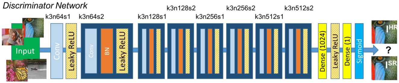
Fig 13: SRGAN Disrcriminator as described in paper
Source: Click here
|
|
|
|
تقدر تشوف كود الـdiscriminator بالكامل هنا.
الـdataset المستخدمة في الـtraining
الميزة في الـsuper resolution هو إننا نقدر نكوّن dataset بشكل سهل ومباشر، ممكن أجمّع صور high resolution من أي مكان وأطبّق عليها down sampling عشان اطلع منهم صور low resolution، الـPaper الخاصة بـSRResNet و SRGAN عملت كده وطبّقت bicubic downsampling على جزء من ImageNet dataset عشان تطلع منها صور low resolution.
لكن الـpaper الخاصة بـEDSR استخدمت dataset مختلفة وهي DIV2K ، الـdataset دى مجهزة ومصممة خصيصاً لمشكلة الـsuper resolution، تحتوي على 1000 صورة بـresolution 2k مقسّمة إلى 800 صورة training، و100 صورة validation، و100 صورة testing. الـdataset موجود منها أكتر من نسخة بناء على الـscaling factor والـdownsampling الى هتختاره، لذلك إحنا هنشتغل عليها و هنختار scaling factor= 4 و bicubic downsampling.
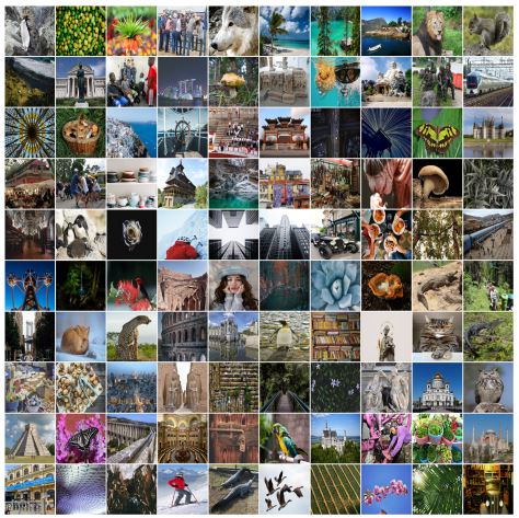
Fig 14: DIV2K validation set
Source: Click here
ممكن تشوف السكربت الى بيحمل الـdataset هنا، أما بالنسبة للـpreprocessing فكل الى عملناه هو إننا قسمنا كل صورة high resolution لمجموعة صور بحجم 256×256 وكل صورة low resolution لمجموعة صور بحجم 64×64 عشان يكون الـscaling factor 4 زى ما حددناه، ممكن تشوف سكربت الـpreprocessing هنا. إجمالي عدد الصور بعد الـpreprocessing تخطّى 28,000 صورة وهو عدد كافي للـtraining.
Model training
قبل ما نعمل training لازم نعمل data loader الأول بيقرأ كل batch من الـdisk، لإن حجم الdataset ممكن يكون كبير على الـRAM، الـdata loader هيكون عبارة عن class بتـinherit من tensorflow.keras.utils.Sequence، هنعرف الـconstructor بتاعها كالآتي:
|
|
لاحظ إن الـconstructor بياخد الـpath الموجود فيه الـdata، وهنا هو بيفترض إن الـdata متقسمة لفولدرين في الـpath ده: HR بيتحوى الصور الـhigh resolution، وLR بيحتوي الصور الـlow resolution، كمان بيفترض إن كل صورة high resolution والمناظر لها في الـlow resolution لهم نفس الاسم أو على الأقل موجودين بنفس الترتيب في الفولدرين، لذلك لازم تتأكد من كده عشان الداتا تدخل بشكل صحيح للموديل.
باقي الـarguments الى في الـconstuctor استخدامها واضح من اسمها: الـbatch_size هو عدد الصور في كل batch، و shuffle عشان لو عايز أعمل shuffle للداتا بعد كل epoch، و load_all_data لو عايز أحط الداتا كلها في الـRAM لو عندي مساحة تكفيها
|
|
__len__ بنعرّفها عشان نحدد عدد الـbatches per epoch، وهو عدد الصور الكلي على الـbatch_size.
on_epoch_end بنعرّف فيها الى احنا عايزينه يحصل بعد كل epoch، هنا هنعمل shuffle للـdata بعد كل epoch لو كنا محددين إن shuffle = True في الـ__init__.
|
|
__getitem__ هى أهم method في الـdata loader، وفيها بنقرأ الداتا من الـdisk (أو من الـRAM) ونرجعها للموديل، وفي الـmethod دى أحنا ممكن نعمل أي preprocessing إضافي على الداتا بعد ما نقرأها وقبل ما نرجعها للموديل، لكن لازم تاخد في الاعتبار إن ده هيأثر على الـtraining time بشكل كبير لو الـpreprocessing الى بتعمله تقيل، هنا احنا مش بنعمل preprocessing وبنرجع الـdata مباشرة للموديل.
load_patch مش method أساسية في الـdata loader لكننا هنعرّفها عشان نستخدمها واحنا بنعمل training للـGAN وهنشوف استخدامها في الـtraining.
ممكن تشوف كود الـdata_loader بالكامل هنا
بعد ما جهزنا الـdataset والـloader الخاص بها الأن ممكن نعمل الـtraining cycle.
في البداية هنعمل SrganTrainer class ونجهز كل مستلزمات الـtraining:
|
|
في الـconstructor هنعرّف الـlow resolution shape والـhigh resolution shape، هنديله الـgenerator والـdiscriminator وهنعرّف optimizer خاص بكل موديل، الـlearning rate المستخدم في الـpaper هو 1e-4 لأول 100,000 mini-batch وبعد كده بيقل لـ1e-5، لكن الى استخدمته هنا هو learning rate ثابت فقط.
هنعرّف الـdata loader ونديله الـpath الموجود فيه الداتا، وأخيرا هنعرف بعد الـvariables الى هنستخدمهم في حسابات الـloss لكل موديل، أول حاجة هنعرفها هي الـVGG network الى هنستخدمها في حساب الـcontent loss:
|
|
هنستخرج feature maps من الـconv layer رقم 4 قبل الpooling layer رقم 5 من VGG19، وهى دى الى هنحسب بيها الـcontent loss:
|
|
الـadversarial loss والـdiscriminator loss ممكن نحسبهم عن طريق binary cross entropy كالآتي:
|
|
الخطوة التالية هي تدريب الموديل بشكل مستقل (سواء كان SRResNet أو EDSR) الـEDSR بيحتاج وقت أقل في الـtraining والـevaluation بتاعه أفضل لذلك هنسخدمه مكان الـSRResNet.
|
|
لاحظ إن لازم الـgenerator يكون trained لوحده باستخدام MSE أو MAE الأول قبل ما يتم تدريبه في الـGAN، السبب هو إن مهمة الـgenerator تعتبر أصعب بكتير من الـdiscriminator لإنه بيحاول يكوّن صورة كاملة، على عكس الـdiscriminator الى بيحاول يدي لكل صورة score بين 0 و 1 فقط، فلو لو جربت استخدم untrained generator هلاقي إن الـdiscriminator بيتعلم أسرع منه بكتير والgenerator مش هيقدر يتعلم كويس، لذلك خطوة الـpre-training مهمة قبل الـGAN
عشان نعمل training للـGAN هنعمل forward pass، هنحسب الـlosses ، وأخيراً هنعمل backward pass عشان نحسب الـgradients ونعمل update للـweights كالآتي:
|
|
آخر حاجة هى إننا نكرّر الخطوة دى عدد معيّن من الـsteps لحد ما نوصل لنتيجة جيّدة، الـpaper عملت training لـ200,000 step لكن ممكن توقف الـtraining قبلها لو وصلت لنتيجة جيدة:
|
|
ممكن تشوف كود الـtraining بالكامل هنا
وآخيرا آخر خطوة هى إننا نبدأ الـtraining:
|
|
النتيجة النهائية للـEDSR بعد تدريبه داخل الـSRGAN موضّحة في Figure 15، لاحظ التفاصيل الإضافية الموجودة في الناتج، مع اختفاء الـblurring الواضح الى كان بيظهر في ناتج الموديل السابق.
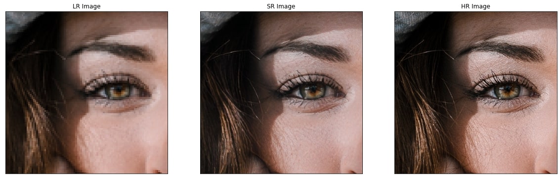
Fig 15: SRGAN Result (middle), compared to input (left) and original image (right)
مقارنة بين نتائج الـmodels
الـmetrics المستخدمة في تقييم أي super resolution model هما الـPSNR والـSSIM، لكن زى وضحنا سابقاً فالـPSNR الأكبر لا يعني جودة صورة أفضل، ولذلك الـpaper اعتمدت على metric جديد وهو الـmean opinion score (MOS)، وهو معتمد على تقييم الناس لنتيجة الموديل، كل مشترك بيتعرض عليه أكتر من نسخة من كل صورة لكن بدون اخباره بالموديل المستخدم في تكوينها وكل الى عليه هو اعطاء كل صورة درجة من 5.
إحنا قررنا نعمل نفس التجربة عشان نحسب الـMOS لكل موديل وعملنا استبيان شارك فيه 67 شخص، كل مشترك اعطى تقييم لأربع نسخ من كل صورة من 13 صورة استخدمناهم في الاستبيان باجمالى 871 تقييم لكل model، النسخ الموجودة من كل صورة كانت ناتجة من bicubic interpolation, EDSR, EDSR(SRGAN), والصورة الـoriginal. وكانت النتائج كالآتي:
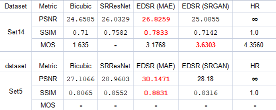
Table 1: Models Evaluation metrics on Set14 and Set5
واضح من النتائج إن EDSR هو أفضل موديل من حيث الـPSNR والـSSIM، لكن تقيييمات المشاركين فضّلت ناتج الـSRGAN عليه لإن التفاصيل فيه أفضل وبالتالي كان أقرب من باقي الـmodels للصورة الأصلية. في الـfigures التالية هستعرض نواتج كل model جنب بعض للمقارنة:
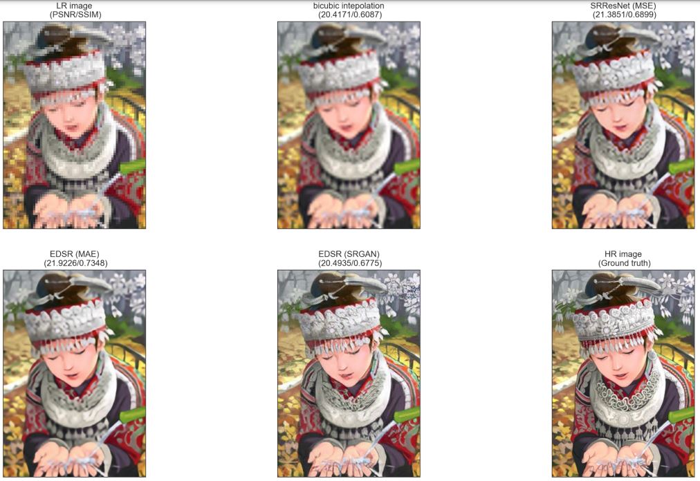
Fig 16: Result on Painting image from Set14
View full image
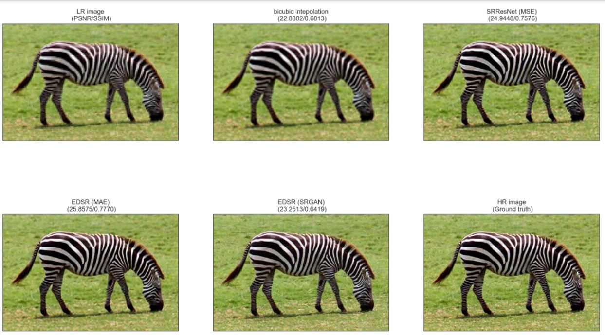
Fig 17: Result on Zebra image from Set14
View full image
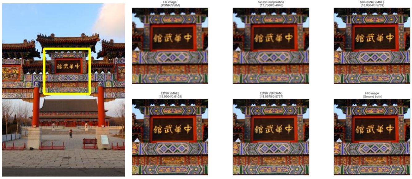
Fig 18: Result on image 0826 from DIV2K
View full image
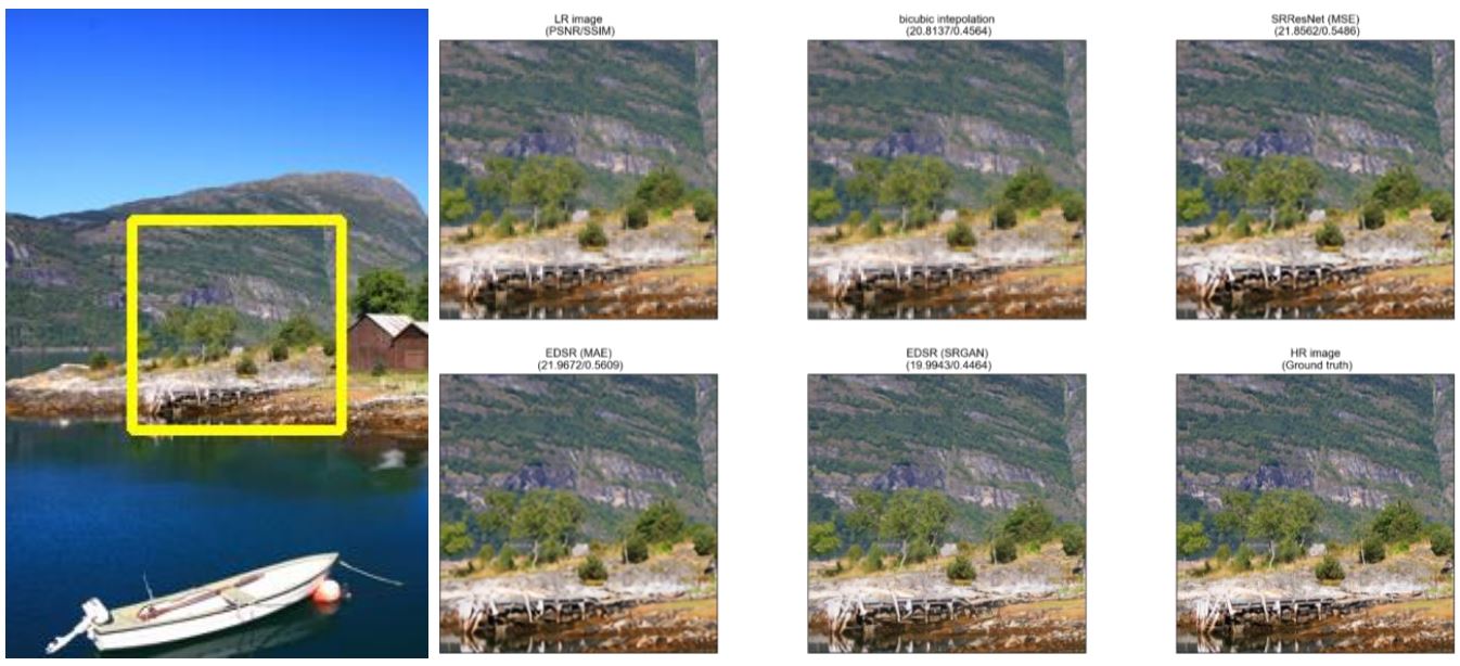
Fig 19: Result on image 0808 from DIV2K
View full image
- Deep Learning for Single Image Super-Resolution: A Brief Review
- Image Super-Resolution Using Deep Convolutional Networks
- Photo-Realistic Single Image Super-Resolution Using a Generative Adversarial Network
- Enhanced Deep Residual Networks for Single Image Super-Resolution
- Super-Resolution.Benckmark
- DIV2K dataset: DIVerse 2K resolution high quality images
- Peak signal-to-noise ratio (PSNR)
- Structural Similarity Index Measure (SSIM)